Getting Started
Installation
pip install --upgrade findiff
Derivatives
First Derivatives
The first derivative along the 0-th axis (”\(x_0\)-axis”),
can be defined by
from findiff import Diff

d_dx = Diff(0, dx)
The first argument is the axis along which to take the partial derivative. The second argument is the spacing of the (equidistant) grid along that axis.
Accordingly, the first partial derivative with respect to the k-th axis
is
Diff(k, dx_k)
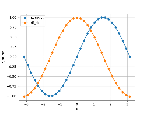
Let’s initialize a one-dimensional array f with some values, for example:
import numpy as np
x = np.linspace(-np.pi, np.pi, 100)
dx = x[1] - x[0]
f = np.sin(x)
and calculate the first derivative with respect of the zeroth axis.
Diff objects behave like operators, so in order to apply them, you can
simply call them on a numpy ndarray of any shape:
d_dx = Diff(0, dx)
df_dx = d_dx(f)
Now df_dx is a new numpy array with the same shape as f containing the
first derivative with respect to the zeroth axis:
Higher Derivatives
The n-th partial derivatives, say with respect to \(x_k\),
can be written by exponentation:
Diff(k, dx_k) ** n
A mixed partial derivatives like
can be written by “multiplication”:
Diff(0, dx)**2 * Diff(1, dy)
General Differential Operators
Diff objects can be combined to describe general differential
operators. For example, the wave operator
can be written as
1 / c**2 * Diff(0, dt)**2 - Diff(1, dx)**2
if the 0-axis represents the t-axis and the 1-axis the x-axis.
This works both for constant and variable coefficients.
Finally, multiplication of two FinDiff objects means chaining differential
operators, for example
or in findiff:
d_dx = Diff(0, dx)
d_dy = Diff(1, dy)

(d_dx - d_dy) * (d_dx + d_dy)
Accuracy Control
By default, findiff uses finite difference schemes with
second order accuracy in the grid spacing. Higher orders can be selected
by setting the keyword argument acc, e.g.
Diff(0, dx, acc=4)
for fourth order accuracy.
Finite Difference Coefficients
findiff uses finite difference schemes to calculate numerical derivatives.
If needed, the finite difference coefficients can be obtained from the
coefficients function, e.g. for second derivative with second order
accuracy:
from findiff import coefficients
coefficients(deriv=2, acc=2)
which yields
{'backward': {'accuracy': 2,
              'coefficients': array([-1.,  4., -5.,  2.]),
              'offsets': array([-3, -2, -1,  0])},
 'center': {'accuracy': 2,
            'coefficients': array([ 1., -2.,  1.]),
            'offsets': array([-1,  0,  1])},
 'forward': {'accuracy': 2,
             'coefficients': array([ 2., -5.,  4., -1.]),
             'offsets': array([0, 1, 2, 3])}}
Matrix Representations
For a given FinDiff differential operator, you can get the matrix representation using the matrix(shape) method, e.g.
x = [np.linspace(0, 6, 7)]
d2_dx2 = Diff(0, x[1]-x[0]) ** 2
u = x**2

mat = d2_dx2.matrix(u.shape)  # this method returns a scipy sparse matrix
print(mat.toarray())
yields
[[ 2. -5.  4. -1.  0.  0.  0.]
 [ 1. -2.  1.  0.  0.  0.  0.]
 [ 0.  1. -2.  1.  0.  0.  0.]
 [ 0.  0.  1. -2.  1.  0.  0.]
 [ 0.  0.  0.  1. -2.  1.  0.]
 [ 0.  0.  0.  0.  1. -2.  1.]
 [ 0.  0.  0. -1.  4. -5.  2.]]
Of course this also works for general differential operators.
Stencils
Automatic Stencils
When you define a differential operator in findiff, it automatically chooses suitable stencils to apply on a given grid. For instance, consider the 2D Laplacian
which can be defined (in second order accuracy here) as
laplacian = Diff(0, dx) ** 2 + Diff(1, dy) ** 2
When you then apply the Laplacian to an array, findiff applies it to all grid points. So depending on the grid point point, findiff chooses on or the other stencil.
You can inspect the stencils for a differential operator by calling
its stencil method, passing the shape of the grid
laplacian.stencil(f.shape)
This returns
{('L', 'L'): {(0, 0): 4.0, (0, 1): -5.0, (0, 2): 4.0, (0, 3): -1.0, (1, 0): -5.0, (2, 0): 4.0, (3, 0): -1.0},
 ('L', 'C'): {(0, -1): 1.0, (0, 1): 1.0, (1, 0): -5.0, (2, 0): 4.0, (3, 0): -1.0},
 ('L', 'H'): {(0, -3): -1.0, (0, -2): 4.0, (0, -1): -5.0, (0, 0): 4.0, (1, 0): -5.0, (2, 0): 4.0, (3, 0): -1.0},
 ('C', 'L'): {(-1, 0): 1.0, (0, 1): -5.0, (0, 2): 4.0, (0, 3): -1.0, (1, 0): 1.0},
 ('C', 'C'): {(-1, 0): 1.0, (0, -1): 1.0, (0, 0): -4.0, (0, 1): 1.0, (1, 0): 1.0},
 ('C', 'H'): {(-1, 0): 1.0, (0, -3): -1.0, (0, -2): 4.0, (0, -1): -5.0, (0, 0): 0.0, (1, 0): 1.0},
 ('H', 'L'): {(-3, 0): -1.0, (-2, 0): 4.0, (-1, 0): -5.0, (0, 0): 4.0, (0, 1): -5.0, (0, 2): 4.0, (0, 3): -1.0},
 ('H', 'C'): {(-3, 0): -1.0, (-2, 0): 4.0, (-1, 0): -5.0, (0, -1): 1.0, (0, 0): 0.0, (0, 1): 1.0},
 ('H', 'H'): {(-3, 0): -1.0, (-2, 0): 4.0, (-1, 0): -5.0, (0, -3): -1.0, (0, -2): 4.0, (0, -1): -5.0, (0, 0): 4.0}}
In the interior of the grid (the :code:`(‘C’, ‘C’) case), the stencil looks like this:
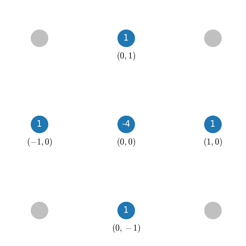
The blue points denote the grid points used by the stencil, the tu ple below denotes the offset from the current grid point and the value inside the blue dot represents the finite different coefficient for grid point. So, this stencil evaluates the Laplacian at the center of the “cross” of blue points. Obviously, this does not work near the boundaries of the grid because that stencil would require points “outside” of the grid. So near the boundary, findiff switches to asymmetric stencils (of the same accuracy order), for example
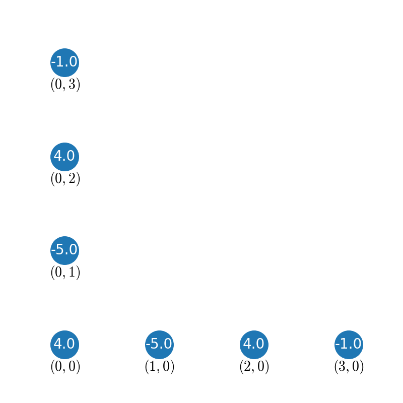
for a corner ('L', 'L'), or
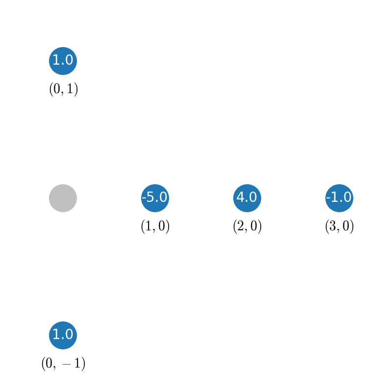
for the left edge ('L', 'C').
The stencil method works for grids of all dimensions and not just two. But of course,
it is not easy to visualize for higher dimensions.
While FinDiff object act on complete arrays, stencils can be applied
to individual grid points, if you just need a numeric derivative evaluated
at one point. For instance,
x = y = np.linspace(0, 1, 101)
X, Y = np.meshgrid(x, y, indexing='ij')
f = X**3 + Y**3

stencils = laplacian.stencil(f.shape)
stencils.apply(f, (100, 100)) # evaluate at f[100, 100]
returns 12, as expected. stencil returns a list of stencils and
when calling apply, the appropriate stencil for the selected grid point
is chosen. In the example, it chooses a stencil for the corner point.
Stencils From Scratch
There may be situations when you want to create your own stencils and do not
want to use the stencils automatically created by FinDiff objects.
This is mainly for exploratory work. For example, you may wonder, how the
coefficients for the 2D Laplacian look like if you don’t use the cross-shaped
stencil from the previous section but rather an x-shaped one:
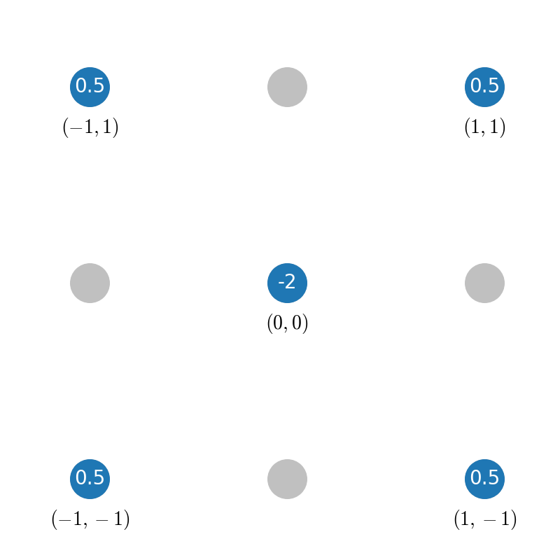
This can easily be determined with findiff by using the Stencil class directly:
offsets = [(0, 0), (1, 1), (-1, -1), (1, -1), (-1, 1)] # x-shaped offsets
stencil = Stencil(offsets, {(2, 0): 1, (0, 2): 1})
returns
{(0, 0): -2.0, (1, 1): 0.5, (-1, -1): 0.5, (1, -1): 0.5, (-1, 1): 0.5}
The second argument of the Stencil constructor defines the derivative operator:
{(2, 0): 1, (0, 2): 1}
corresponds to